The p-y curves procedure for cohesive soils can be summarized in the following steps:
| Undrained Shear strength, cu [kN/m2] | ε50 [-] |
|---|---|
| <12 | 0.02 |
| 12-24 | 0.02 |
| 24-48 | 0.01 |
| 48-96 | 0.006 |
| 96-192 | 0.005 |
| >192 | 0.004 |
Matlock (1970) conducted full-scale lateral test on 0.3-m diameter steel piles embedded in soft clay deposit in Lake Austin, Texas. Later, API sponsored a study for clay (O’Neill and Gazioglu, 1984), with the purpose to include the pile diameter effects in an alternative clay p-y procedure, known as Integrated Clay P-y Procedure. However, API did not adopt the proposed changes and the Matlock clay criterion remains the API recommended clay p-y procedure.
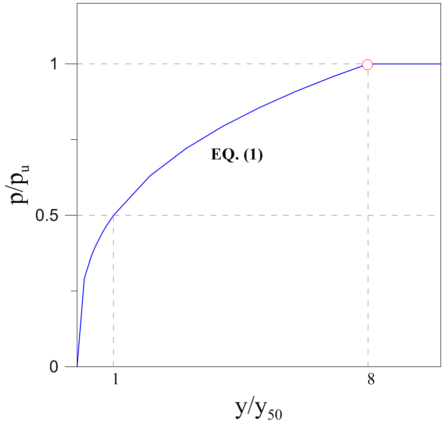
Matlock (1970) proposed a parabolic p-y curve shape (Eq. 1) characterized by a theoretical initial tangent modulus that is infinite at zero deflection. To formulate the initial tangent p-y stiffness, the soil strain, e, has been used. The ultimate capacity of the p-y curve, pu, is strongly dependent to the depth and the diameter (Eq. 2).
The proposed formulation for soft clays in the presence of free water is as follows:


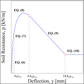
Reese et al. (1975) proposed a p-y curve formulation to represent the response of stiff clays in the presence of free water. This methodology was developed after lateral load tests on two 0.6-m diameter steel piles embedded in stiff clay under water table at Manor, Texas. The proposed curves are composed by five portions (Eq. 4-8) and its shape is presented in Fig. 2. The initial straight line (Eq. 6) has an initial stiffness, Kpy, which is calculated from a coefficient of variation in subgrade modulus with depth (FL-3). Once it has been multiply by depth z, the initial stiffness can be assumed to be independent of pile diameter, b. This assumption is valid only in the case of deflections less than 0.02 inch. At any non-zero deflection values, the secant stiffness will be dependent on both the initial tangent modulus and pu, strongly dependent on diameter (Eq. 9).
The ultimate soil resistance pu and y50 are given by Eq. 4 and 5:

Reese et al.’s p-y curve is composed by five parts, given by the following equations. The initial straight line is given by:
| Average undrained shear strength, ca [kPa] | |||
|---|---|---|---|
| 50-100 | 200-300 | 300-400 | |
| Kpy(static) [MN/m3] | 135 | 270 | 540 |
| Kpy(static) [MN/m3] | 55 | 110 | 540 |
The straight line is followed by two parabolic portions, given by:

The two final straight lines are given by:

As is dimensionless parameter used in static loading and function of the depth and pile diameter.
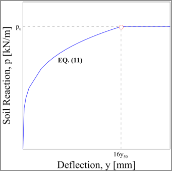
Reese and Welch (1972) proposed a p-y curve formulation stiff clays with no free water after conducting lateral load tests on a 0.76-m diameter bored pile in Houston, Texas. The shape of the curves (Fig. 3) is the same as Matlock (1970), but stiffer due to the use of the forth degree of parabolic relationship between p and y, which is as follows:
The value of p/pu remains constant beyond y = 16y50.
The procedure is for short-term static loading and for cyclic loading. The ultimate soil resistance is given by the smallest results of the following two equations:

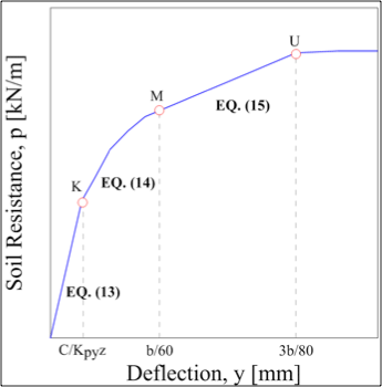
The p-y curve is composed by four parts: an initial straight line (13), a parabolic portion (14), and a final straight line (15):
with Kpy, depending on f (Table 3). As and Bs are dimensionless parameters used in static loading and function of the depth and pile diameter.
Table 3. Initial stiffness, Kpy, according to Reese, Cox and Koop 1974.| Loose (f<30°) | Medium (30≤f<36°) | Dense (f≥36°) | |
|---|---|---|---|
| Kpy(below water table) [MN/m3] | 5.4 | 16.3 | 34 |
| Kpy(above water table) [MN/m3] | 6.8 | 24.4 | 61 |
 ;
;
 ;
;
 ;
;
The value of p remains constant after ![]() .
.
Subsequently, parallel to the study conducted by O’Neill and Gazioglu (1984) in clay, API also sponsored a study for sand by O’Neill and Murchinson (1983) with the purpose to simplify the original Reese’s procedure without introducing fundamental changes (Lam, 2009). The only modification regards the change of the original parabolic curve shape into a hyperbolic one. Otherwise the two methods are identical, as demonstrated by the identical initial tangent stiffness and the ultimate capacity in the hyperbolic curve. Moreover, the lengthy equations for determining the ultimate soil pressure were simplified by the use of three coefficients C1, C2 and C3 as a function of the friction angle (Eq. 19).
The proposed p-y curve parameterization is as follows:
With C1, C2, C3 = dimensionless coefficients related to f; kpy is determined as function of f.
There are no available recommendations on developing p-y curves for soil with cohesion and friction angle that are generally accepted. Generally, in design, the soil is classified in only two different types: cohesive or cohesionless. In the practice, this simplification leads to a significantly conservative design in the case of cemented soil or silt, which always neglects the soil resistance from the cohesion component (Juirnarongrit et al. 2005).
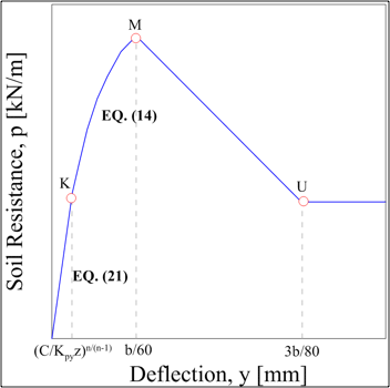
Evans and Duncan (1982) proposed the following procedure for developing p-y curves in silty soils. The ultimate soil resistance is given by:
With puf is the smallest of (12), whereas puc is the smallest of (1). The dimensionless parameter, As, is from Reese, Koop and Cox (1974). This p-y curve is composed by an initial straight line (21), a parabolic portion (14) and two straight lines.
The value of p remains constant beyond ![]() .
.
Johnson et al. (2006) studied the response of loess soils and proposed the following step procedure:
The following symbols are used: